Summary
In this post, we cover descriptions of Bayes Theorem and Naive Bayes. We then use Naive Bayes to classify Wikipedia comments as harmful or harmless. The model created detects 58% of harmful comments in the test data. In future posts, we improve the model by using more features and different classification models.
Introduction
Most of us find the internet entertaining and resourceful, but sometimes we come across perjoratives in various forums. Text classification can automate the identification of harmful comments hence preventing them from been posted or deleting them as soon as they are posted, making the internet safe and friendly for all of us. In this post, we train a Naive Bayes classifier to identify harmful comments. The data is from this Kaggle Toxic Comment Classification Challenge.
Let’s get started.
Explore the data
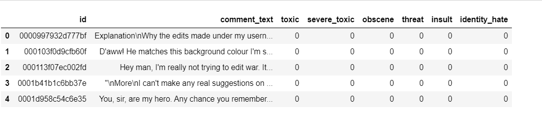
Training data, as provided by Kaggle, has 159571 rows and 8 variables. The variables are as follows:
* id - unique identifier of each comment
* comment_text - the actual comments from wikipedia
* toxic - binary column taking 1 for toxic comments and 0 otherwise
* severe_toxic - binary column taking 1 for severe toxic comments and 0 otherwise
* obscene -binary column taking 1 for obscene comments and 0 otherwise
* threat - binary column taking 1 for threat comments and 0 otherwise
* insult - binary column taking 1 for insult comments and 0 otherwise
* identity_hate - binary column taking 1 for identity hate comments and 0 otherwise
The Kaggle training data looks as shown below:
 . The Kaggle testing data contains only the id and comment_text columns.
The Kaggle Challenge is a multilabel classification (a comment is assigned more than one toxicity level - toxic, severe toxic etc), but in this post we will focus on just whether a comment is harmful or not. We create a column that indicates whether a column is harmful (takes value 1 in any of the 5 levels of toxicity) as shown below:

The percentage of harmful comment is only 10% making this a highly imbalanced dataset.
 .
.
We then split the data into two to create our own training and testing datasets.

Building a simple classification model with Naive Bayes
Going by the fact that words used are the most obvious indicator of whether a comment is harmless or harmful, we will build a simple Naive Bayes model that will classify comments as harmful or otherwise. Naive Bayes is one of my favourite machine learning algorithms as I find it simple and intuitive.
My understanding of Naive Bayes
Say you wake up in the morning and are deciding on something to wear. For simplicity, let us assume you only have 5 sets of clothes, some lighter than others, but you like them equally and the weather has been alternating between cold and warm days. At first, your curtains are drawn closed so you have no idea whether its cloudy or sunny. The probability of picking any of set of clothes is 0.2 (1/5) as you have 5 sets and you like all pairs equally. You decide to draw the curtain open, and voila, it’s sunny. Suppose that of your 5 pairs of clothes, 3 pairs are lighter and hence more comfortable for warm days.Given how sunny it looks, you will shift your attention from all the 5 sets of clothes to the 3 sets of light clothes. Now, the probability of picking any of the 3 sets of clothes is 0.33 (1/3) and the probability of picking any of the other 2 sets of clothes is 0.
Mathematics of Naive Bayes
Naive Bayes is an application of Bayes theorem that states:
P(H|A) = P(A|H)P(A)/P(H)Let’s take a different example. Suppose you have 5 wikipedia comments and you know that 2 of them are harmful meaning that the probability that any comment picked at random, without looking at its wording, is harmful is 0.2 (1/5). Let’s call this P(H).
Looking at the comments, you realize that 3 of them contain the word “ass” hence the probability that any randomly picked comment contains the word “ass” is 0.33 (1/3). Let’s call this P(A).
Further looking at the comments reveals that of the 2 harmful comments, only 1 contains the word “ass” so the probability that a comment contains the word ass when we know that the comment is harmful is 0.5 (1/2). We call this P(A|H).
Let’s define P(H|A) as the probability that a comment is harmful when we know that it contains the word “ass” such that we calculate P(H|A) as 0.5 * 0.2/0.33 = 0.3. Now we know that if we pick any comment and glimpse only the word “ass” in it, it is 30% likely to be a harmful comment. 30% is higher than our original estimate of 20% when we picked a comment and did not have a look at any of its wording. The knowledge that the comment contains the word “ass” makes us know that it is more likely to be a harmful comment.
Naive Bayes applies Bayes Theorem, but with a few tweaks to make it more robust. In this case, Naive Bayes will find evidence of a comment been harmful or harmless based on the words used. To learn more about Naive Bayes, please read Chapter 4 of Machine Learning with R by Brett Lantz which offers a simple and comprehensive explanation.
Implementation of Naives Bayes using Python’s Scikit Learn
Step 1: Clean the comments
We only want to use words for classification thus we need to clean the comments to ensure that we remain mostly with meaningful words.We start by cleaning/uniformizing the comments by changing the comments to lower case and removing characters that are not letters.
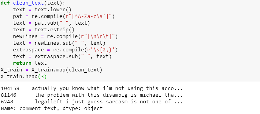
Then we remove english stopwords, words with less than 3 characters and we lemmatize each word in the comments.

Step 2: Transform the comments into a vector
As earlier mentioned, we will use words as the predictors of harmful comments in our model thus we need to transform the comments into a vector such that each comment is a row and each unique word is a column. Two of the commonly used vectors in Sklearn are:
- Count Vectors implemented with CountVectorizer()
A count vector is a matrix in which each coment is a row, each column is a unique word from the collection of sentences and each cell value is the number of times a particular word appears in a comment.
Say you have the following sentences:
- the cat is black and white
- the dog is white and brown
Then the count vector looks as shown below:

- TFIDF Vectors implemented with TfidfVectorizer()
Depending on the context, you may have words that appear in almost all comments such as determiners, pronouns, prepositions and contextual vocabularies. These common words can biase your dataset (make it seem like they have greater predictive power than they actually do). This is where IDF comes in to balance things out by assigning less weight to frequently occurring words and more weight to rarely occurring words.
TF represents term frequency - the number of times a word appears in a comment(what we got in count vector above). Sometimes term frequency is normalized by calculating it as:
= Number of times a word appears in a comment/Total number of words in a comment
IDF represents Inverse Document Frequency and is calculated as:
= log(Number of comments/Number of comments in which a particular word appears)From this formula you see that a greater denominator will result into a smaller figure. From our sentences above, we calculate the IDF of “black” as:
= log(2/1) as there are 2 sentences and "black" appears in 1 sentence.TFIDF is the product of TF and IDF. Sklearn documentation offers a very good explanation of count and tfidf vectors here. We will use TFIDF vectors:

Step 3: Build the model

Step 4: Predict whether comments in our test data are harmful or not
We first transform the comments in the test data as we transformed those in the training data then apply our classification model onto the test data comments and evaluate how well our model does.
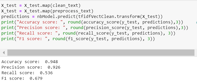
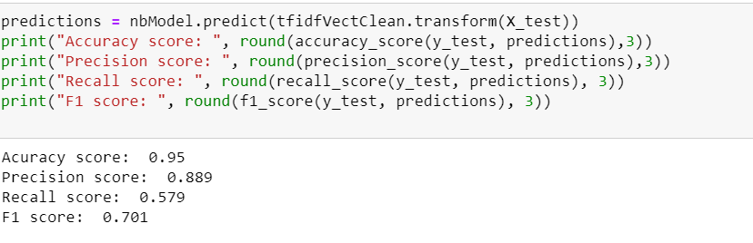
As the data is highly imbalanced, accuracy is a poor metric because if you guess that a comment is harmless, 90% of the time you will be correct. We will therefore use precision, recall and F1 score as our evaluation metrics. As a reminder, earlier on we assigned 1 to comments that are harmful thus harmful is our positive class while harmless is the negative class.
Precision is the proportion of comments classified by our model as harmful that are actually harmful. Precision is calculated as:
            TP/(TP + FP) where TP (True Positive) means the number of comments in the positive (harmful) class that are predicted by the model to be positive.

                               FP (False Postive) means the number of comments in the negative (harmless) class that are predicted by the model to be positive.
Our model classifies 92% of harmful comments as harmful meaning that of all the comments that were predicted as harmful, 8% were actually harmless.
Recall is the proportion of harmful comments that were classified by our model as harmful and is calculated as:
TP/(TP + FN) where FN (False negative) means the number of comments that are in the positive (harmful) class but are predicted by the model to be negative.
A recall of 54% means that the model detected only 54% of harmful comments and incorrectly classified 46% harmful comments as harmless. We want to flag off as many harmful comments as possible thus recall is the most important metric and we need it to be way higher.
F1 score is a composite of precision and recall therefore we also need it to increase as we increase the recall.
Step 5: Improve the model by trying different parameters
TfidfVectorizer() and MultinomialNB() take a couple of parameters that can help with fine tuning our model (visit the links to see explanation of all parameters). In this example, we use alpha from MultinomialNB(), min_df, sublinear_tf, ngram_range, use_idf and smooth idf from TfidfVectorizer() to improve our recall score.
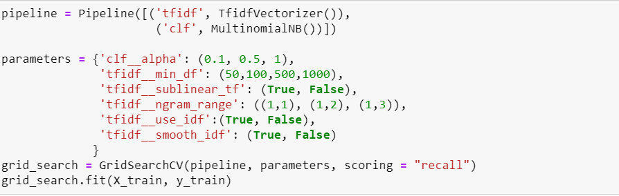

Using the best parameters from the grid search results, we create our final Naive Bayes model as:
The test data recall score improved by only 4% reaching 58%. In the next post, we will try to improve this score by using feature engineering.
Data source: https://www.kaggle.com/c/jigsaw-toxic-comment-classification-challenge/data
References:
Machine Learning with R by Brett Lantz Chapter 4: Probabilistic Learning – Classification Using Naive Bayes
Building Machine Learning Systems with Python by Willi Richerto and Luis Pedro Cooelho Chapter 6
https://towardsdatascience.com/naive-bayes-intuition-and-implementation-ac328f9c9718
https://scikit-learn.org/stable/modules/generated/sklearn.naive_bayes.MultinomialNB.html
Tools:
- R
- Python
#rstats #naivebayes #nlp #flask