In the previous post, we used words to classify Wikipedia comments as harmful or harmless. In this post, we will create a few features from the comments and build another classification model.
To explore features, we will use R as I prefer using R ggplot2
We will start by reading Kaggle’s training dataset, create column “harmful” then select columns “comment_text” and “harmful”.
library(dplyr)
library(caTools)
library(ggplot2)
library(gridExtra)
library(stringr)
library(ngram)
library(tm)
train <- readRDS("Kaggle-Toxic-Comment-Challenge/Data/train.rds")
train$comment_text = as.character(train$comment_text)
train$toxicity_score = rowSums(train[,3:8])
train$harmful = as.factor(if_else(train$toxicity_score == 0, 0, 1))
train = train %>%
select(comment_text, harmful)
head(train$comment_text,2)## [1] "Explanation\nWhy the edits made under my username Hardcore Metallica Fan were reverted? They weren't vandalisms, just closure on some GAs after I voted at New York Dolls FAC. And please don't remove the template from the talk page since I'm retired now.89.205.38.27"
## [2] "D'aww! He matches this background colour I'm seemingly stuck with. Thanks. (talk) 21:51, January 11, 2016 (UTC)"Now we create our own training and testing datasets:
train_sub = sample.split(train$harmful, SplitRatio = 7/10)
new_train = train[train_sub,]
new_test = train[!train_sub,]
We create new features based on our new training dataset and explore their relationships with column “harmful”. As we will be creating numeric features, we create a function to plot density and box plots.
Length of comments: Number of characters
We would expect that harmful comments would be, on average, shorter than harmless comments as harmless comments would seek to offer explanations while harmful comments would dive right into attacks. Let’s take a look.
new_train$length_comment = nchar(new_train$comment_text)
new_train %>%
  group_by(harmful) %>%
  summarise(median_length = median(length_comment), mean_length = mean(length_comment))
## # A tibble: 2 x 3
## harmful median_length mean_length
## <fct> <dbl> <dbl>
## 1 0 216 404.
## 2 1 131 310.Mean and median length of harmless comments are greater than those of harmful comments.
Let’s look at distribution of length of comments:
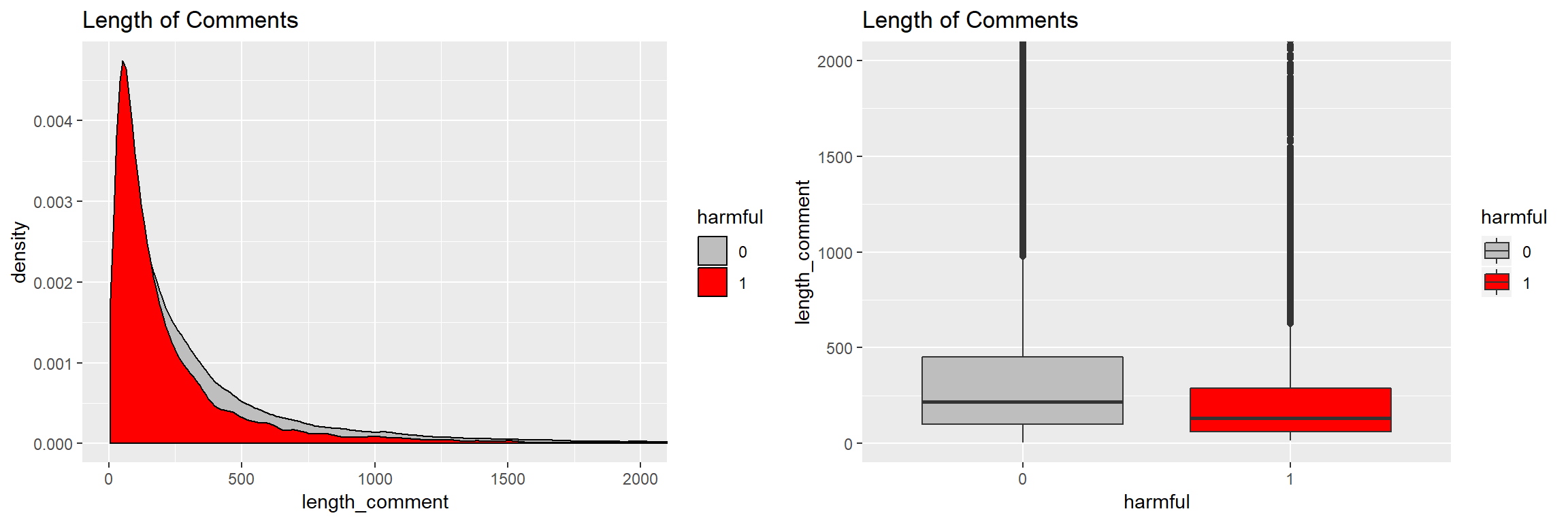
On average, harmful comments are shorter then harmless comments.
Length of comments: Number of words

Similar to number of characters, number of words is lower in harmful comments.
Average length of words
We will use a simplified method to calculate the average length of words in a comment - we will include space in the number of characters.
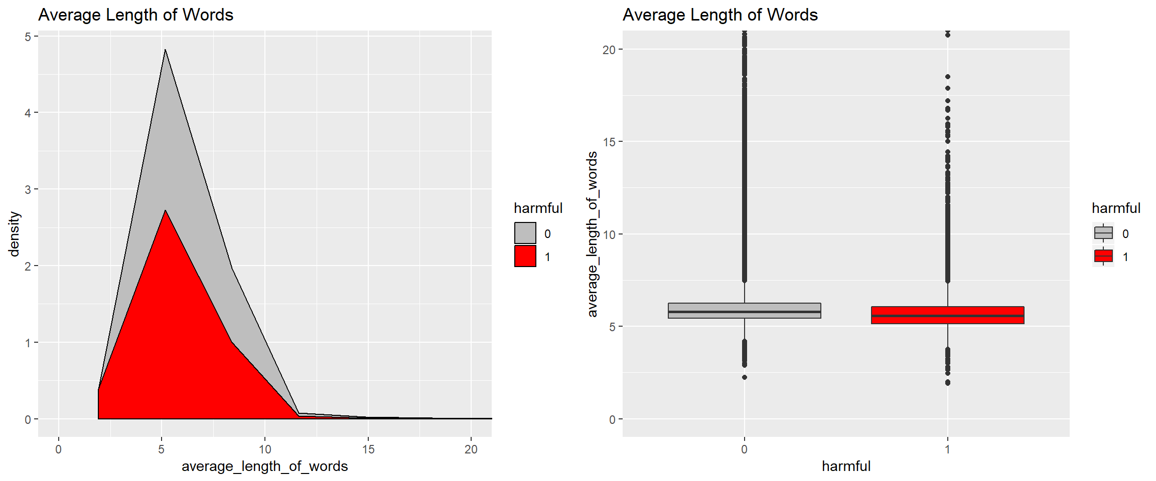
Harmful comments use shorter words on average.
Proportion of repeated words
We would expect that harmless comments use repetition less than harmful comments as harmless comments are aimed at passing a message whereas harmful comments are emotional and use repetitive words for emphasis.
english_stopwords = stopwords("english")

clean_comments = function(x){
  x = tolower(x)
  x = gsub("[0-9]", " ", x)
  x = gsub("\n", " ", x)
  x = gsub("\t", " ", x)
  x = gsub("\\s+", " ", x)
  d = unlist(strsplit(x, " "))
  d = d[!(d %in% english_stopwords) & nchar(d) > 2]
  x = paste(d, collapse = " ")
  x = gsub("[^a-z']", " ", x)
  x = gsub("\\s+", " ", x)
  return(x)
}


remove_repeated_words = function(x){
  x = tolower(x)
  x = gsub("[0-9]", " ", x)
  x = gsub("\n", " ", x)
  x = gsub("\t", " ", x)
  x = gsub("\\s+", " ", x)
  d = unlist(strsplit(x, " "))
  d = d[!(d %in% english_stopwords) & nchar(d) > 2]
  x = paste(unique(d), collapse = " ")
  x = gsub("[^a-z']", " ", x)
  x = gsub("\\s+", " ", x)
  return(x)

}

new_train$cleaned_comments = as.vector(apply(X = new_train[,1, drop = F], MARGIN = 1, FUN = clean_comments))

new_train$unique_word_comments = as.vector(apply(X = new_train[,1, drop = F], MARGIN = 1, FUN = remove_repeated_words))


new_train$number_words_cleaned = as.vector(apply(X = new_train[,6, drop = F], MARGIN = 1, FUN = wordcount))
new_train$number_words_unique = as.vector(apply(X = new_train[,7, drop = F], MARGIN = 1, FUN = wordcount))
new_train$proportion_repeated_words = 1 - new_train$number_words_unique/new_train$number_words_cleaned
new_train[4,]
## comment_text harmful
## 5 You, sir, are my hero. Any chance you remember what page that's on? 0
## length_comment number_of_raw_words average_length_of_words
## 5 67 13 5.153846
## cleaned_comments unique_word_comments
## 5 you sir hero chance remember page on you sir hero chance remember page on
## number_words_cleaned number_words_unique proportion_repeated_words
## 5 7 7 0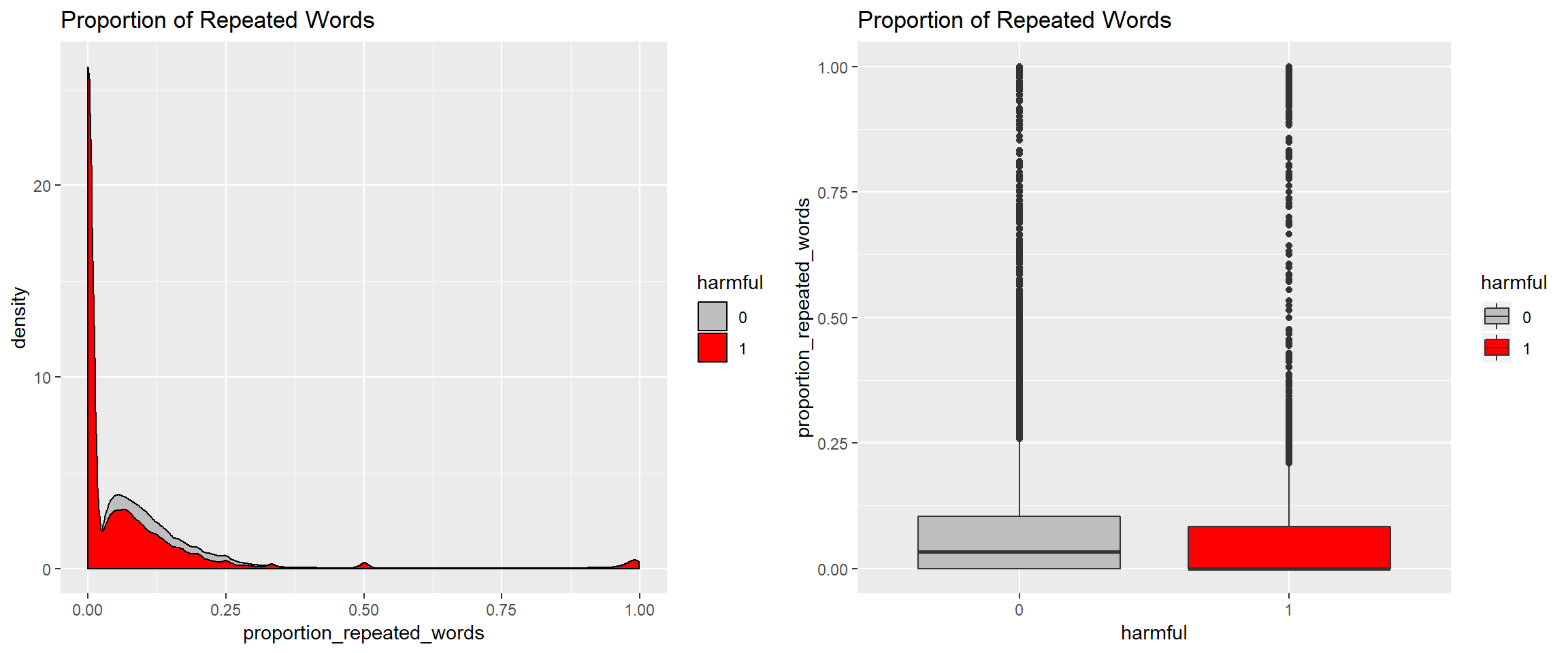
The boxplot contradicts our hypothesis that harmful comments have a higher proportion of repeated words. However, the density plot shows outliers (comments with very high proportion of repeated words) that are dominantly harmful comments. This would be representative of comments whereby the commenter dove into curse words from the first word. Let’s zoom into the outliers:
table(Proportion_repeated_words = new_train$proportion_repeated_words > 0.9, Harmful = new_train$harmful)## Harmful
## Proportion_repeated_words 0 1
## FALSE 100282 11146
## TRUE 41 208ggplot(new_train, aes(x = proportion_repeated_words)) + geom_density(aes(fill = harmful)) + coord_cartesian(xlim = c(0.9, 1)) + ggtitle("Proportion of Repeated Words") + scale_fill_manual(values = c("1" = "red", "0" = "grey"))
A better predictor of harmful comments, in place of proportion of repeated words, an indicator variable indicating whether the proportion of repeated words is very high (higher than say 0.9).
new_train$extreme_repetition = factor(if_else(new_train$proportion_repeated_words > 0.9, 1, 0))Special characters and punctuation in comments
We’ld expect that harmful comments have more special characters and punctuations such as * and exclamation marks. Let’s see if the data supports this.
Clustered exclamation marks
We look at both the number of exclamation marks and the presence of a chain of exclamation marks such as !!!!!!!
new_train$number_exclamation_marks = str_count(new_train$comment_text, "!")
print(tapply(new_train$number_exclamation_marks, new_train$harmful, mean))
## 0 1
## 0.3284268 3.6450960Mean number of exclamation marks in harmful comments is 10 times higher than in harmless comments.

new_train$clustered_exclamation_marks = grepl("!{2,}",new_train$comment_text)
round(prop.table(table(Clustered_exclamation_marks = new_train$clustered_exclamation_marks, Harmful = new_train$harmful), margin = 2),2)
## Harmful
## Clustered_exclamation_marks 0 1
## FALSE 0.99 0.91
## TRUE 0.01 0.099% of harmful comments have clustered exclamation marks as opposed to only 1% of harmless comments.
Asterisks
##          Harmful
## Asterisks    0    1
##     FALSE 0.99 0.97
##     TRUE  0.01 0.03
Asterisks do not appear to be strong features of harmful comments thus we exclude them from our data.
new_train = new_train %>% select(-number_asterisks, -asterisk)Casing of comments - use of all uppercase letters
We would expect that harmful comments would use more uppercase letters as an expression of emotions such as anger.
Proportion of uppercase letters

On average, harmful comments have a higher proportion of upper case letters according to the boxplot. From the density plot, we see the bump around 0.75 indicating a rise in proportion of upper case letters amongst harmful comments. Let us zoom into this:
ggplot(new_train, aes(x = proportion_uppercase_letters)) + geom_density(aes(fill = harmful)) + coord_cartesian(xlim = c(0.7, 1)) + ggtitle("Proportion of Uppercase Letters") + scale_fill_manual(values = c("1" = "red", "0" = "grey"))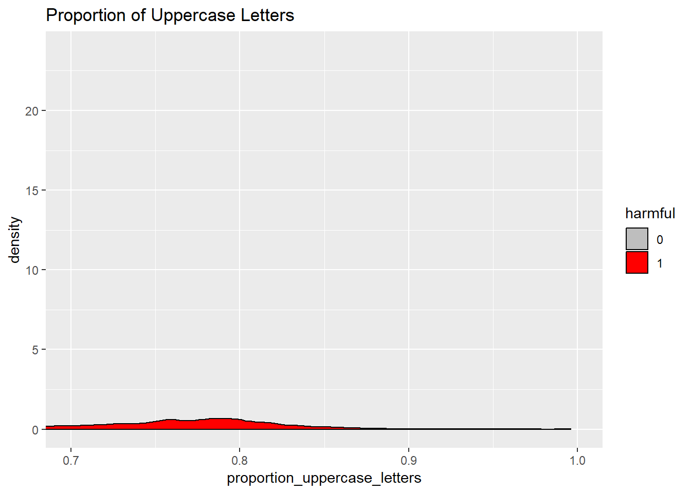
We create a column indicating whether a comment has a very high proportion of uppercase letters.
new_train$extreme_uppercase = factor(if_else(new_train$proportion_uppercase_letters > 0.7, 1, 0))Clustered uppercase letters
new_train$clustered_uppercase = grepl("[A-Z]{5,}", new_train$comment_text)

round(prop.table(table(Harmful = new_train$harmful, clustered_uppercase = new_train$clustered_uppercase), margin = 1) * 100)
## clustered_uppercase
## Harmful FALSE TRUE
## 0 92 8
## 1 79 21Harmful comments are approximately 3 times more likely to have clustered (a chain of at least 5) uppercase letters as compared to harmless comments.
Presence of pronoun “you”
Harmful comments are likely to be targetted at specific individuals and use of “you” is a good indicator that a comment is less likely a general comment than a targetted comment.
new_train$you_comment_text = gsub("you're", "you are", new_train$comment_text, ignore.case = TRUE)
new_train$presence_of_you = grepl(" you ", new_train$comment_text, ignore.case = TRUE)
prop.table(table(Presence_of_you = new_train$presence_of_you, Harmful = new_train$harmful), margin = 2)
## Harmful
## Presence_of_you 0 1
## FALSE 0.5896434 0.4660151
## TRUE 0.4103566 0.5339849More than half (53%) of harmful comments contain the word you. Let us try the number of times you is used in a comment:
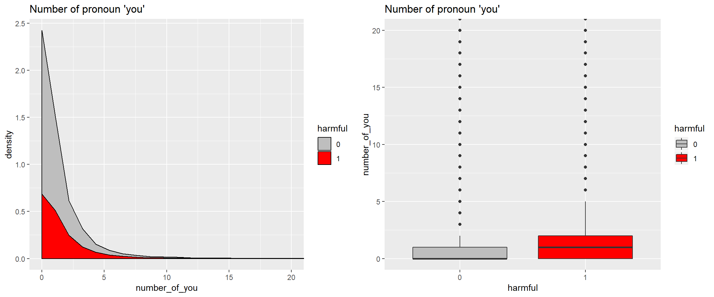
On average, harmful comments have a higher number of “you”s, but harmless comments dominate harmful comments particularly in the lower counts of “you”. To standardize the number of you, we can calculate the proportion of you out of all the words use.

Harmful comments have higher proportions of “you”.
There are many other features we could create from the dataset provided, but for now let us use what we have created. We will create the features in our testing dataset as we did in the training dataset then save the new datasets for use in our classification model.

The additional features improves the recall of the previous model (based on the comments only) by 2% taking the recall to 60%. In the next post, we use deep learning to further improve the recall.
References:
Tools:
- R
- Python